
Du verwendest einen veralteten Browser. Es ist möglich, dass diese oder andere Websites nicht korrekt angezeigt werden.
Du solltest ein Upgrade durchführen oder einen alternativen Browser verwenden.
Du solltest ein Upgrade durchführen oder einen alternativen Browser verwenden.
65 Jahre bemannte Raumfahrt: Die Evolution der orbitalen Mechanik
- Ersteller albertus
- Erstellt am

TomS
Registriertes Mitglied
Er sollte nicht nur lauffähig sondern auch einigermaßen sinnvoll sein. Deswegen bitte Geduld bis morgen. Und ja, selbstverständlich läuft der problemlos, Bibliotheken wie numpy und scipy vorausgesetzt.Wie wäre es mit dem python-Code. Kann ich bei mir laufen lassen (pyCharm als IDE).
TomS
Registriertes Mitglied
Also hier zunächst mal, was ich mir anschaue.
Es geht um SU(2) Rotationen U von Vektoren auf der komplexen projektiven Ebene CP2 (CP1 ist die Riemannsche Zahklenkugel).
Ich betrachte für die Abstandsmessung
,%5Cquad%5C%7CZ%5C%7C%5E2=%7Cz_1%7C%5E2+%5Bz_2%7C%5E2=1)
=(Z_a,Z_a)+(Z_b,Z_b)-2(Z_a,Z_b)=2-2%5Cbar%7BZ%7D_a&space;Z_b=2-2%5Ccos%5Ctheta_%7Bab%7D)
Damit wird aus der euklidischen Norm der Differenz der beiden Vektoren Z_1 und Z_2 ein Abstandsbegriff auf der komplexen projektiven Ebene, die sogenannte Fubini-Study-Metrik
=%5C%7C%7CU_%7Bab%7D%5C%7C%5E2=2-2%5Ccos%5Ctheta_%7Bab%7D)
Ich betrachte Vektoren Z, noch keine Quaternionen Q.
Einen allgemeinen Orbit unter SU(2) Rotationen beschreibe ich mittels
=U(t)%5C,Z_0&space;)
Infinitesimale Rotationen werden durch anti-hermitesche su(2) Generatoren A gemäß
=U(t+dt,t)%5C,Z(t),%5Cquad&space;U(t+dt,t)=e%5E%7BA(t)%5C,dt%7D,%5Cquad&space;A=%5Cdot%7BU%7DU%5E%7B-1%7D)
erzeugt.
Was ich mir später noch anschauen will ist der Geschwindigkeitsbegriff, den man aus den Generatoren A erhält.
Da die gesamte Dynamik in U kodiert ist, sollte für Konvergenzfragen praktisch kein Unterschied zwischen der fundamentalen Darstellungen der SU(2), also der Anwendung der Matrizen U auf Z sowie der adjungierten Darstellung, d.h. der Anwendung auf Elemente der su(2) Algebra bzw., Quaternionen Q bestehen:
=U(t+dt,t)%5C,Q(t)%5C,U%5E%7B-1%7D(t+dt,t))
Außerdem zwingt mich niemand zu irgendwelchen Koordinaten, ich wähle daher die Hopf-Abbildung
,%5Cqquad%5Cleft(z_1,z_2%5Cright)=%5Cleft(e%5E%7Bi%5Cphi_1%7D%5Ccos%5Ctheta,e%5E%7Bi%5Cphi_2%7D%5Csin%5Ctheta%5Cright))
aus der man sofort abliest, dass eine SU(2) Matrix mit

vorliegt.
Der Vorteil dieser Koordinaten liegt darin, dass sie sicher keine Koordinaten-Singularitäten oder andere Artefakte erzeugt sondern explizit und überall glatt ist. D.h. ich habe eine Rahmen, der für sich betrachtet konsistent funktionieren sollte.
Auf der Basis untersuche ich nun vier numerische Lösungsmöglichkeiten der Bewegungsgleichung, nämlich
Zum Code: nicht sehr ausführlich kommentiert, folgt der gerade skizzierten Idee; die Hopf-Abbildung liefert einfach eine "wilde" Testfunktion; Graphiken erklären sich hoffentlich von selbst.
 en.wikipedia.org
 en.wikipedia.org
 en.wikipedia.org
en.wikipedia.org
en.wikipedia.org
Es geht um SU(2) Rotationen U von Vektoren auf der komplexen projektiven Ebene CP2 (CP1 ist die Riemannsche Zahklenkugel).
Ich betrachte für die Abstandsmessung
Damit wird aus der euklidischen Norm der Differenz der beiden Vektoren Z_1 und Z_2 ein Abstandsbegriff auf der komplexen projektiven Ebene, die sogenannte Fubini-Study-Metrik
Ich betrachte Vektoren Z, noch keine Quaternionen Q.
Einen allgemeinen Orbit unter SU(2) Rotationen beschreibe ich mittels
Infinitesimale Rotationen werden durch anti-hermitesche su(2) Generatoren A gemäß
erzeugt.
Was ich mir später noch anschauen will ist der Geschwindigkeitsbegriff, den man aus den Generatoren A erhält.
Da die gesamte Dynamik in U kodiert ist, sollte für Konvergenzfragen praktisch kein Unterschied zwischen der fundamentalen Darstellungen der SU(2), also der Anwendung der Matrizen U auf Z sowie der adjungierten Darstellung, d.h. der Anwendung auf Elemente der su(2) Algebra bzw., Quaternionen Q bestehen:
Außerdem zwingt mich niemand zu irgendwelchen Koordinaten, ich wähle daher die Hopf-Abbildung
aus der man sofort abliest, dass eine SU(2) Matrix mit
vorliegt.
Der Vorteil dieser Koordinaten liegt darin, dass sie sicher keine Koordinaten-Singularitäten oder andere Artefakte erzeugt sondern explizit und überall glatt ist. D.h. ich habe eine Rahmen, der für sich betrachtet konsistent funktionieren sollte.
Auf der Basis untersuche ich nun vier numerische Lösungsmöglichkeiten der Bewegungsgleichung, nämlich
- direkte Berechnung mittels U als Referenz
- lineare infinitesimale Iteration mit expliziter Normierung je Iterationsschritt
- inverse-Cayley-Transformation, wobei diese korrekt bis zweiter Ordnung und zugleich automatisch unitär ist, d.h. ohne Normierung auskommt
- exponentielle Iteration, ebenfalls ohne Normierung
- Koordinatendarstellung von U mittels su(2)-Lie-Algbra, d.h. Rotationswinkel um eine Achse, deren Darstellung mittels Pauli-Matrizen
- adjungierte Darstellung = Wirkung auf auf Quaternionen ~ Elemente der Lie-Algebra
Zum Code: nicht sehr ausführlich kommentiert, folgt der gerade skizzierten Idee; die Hopf-Abbildung liefert einfach eine "wilde" Testfunktion; Graphiken erklären sich hoffentlich von selbst.
Complex projective plane - Wikipedia
Special unitary group - Wikipedia
Hopf fibration - Wikipedia
Fubini–Study metric - Wikipedia
Python:
# SU(2) orbits on the complex unit sphere

# imports ----------

import numpy as np
np.set_printoptions(threshold=np.inf)

import scipy as sci

import matplotlib.pyplot as plt
from matplotlib import use
use('MacOSX')
plt.rc('font', size=8)

import mplcyberpunk
plt.style.use("cyberpunk")


# the model ----------

def hopf_rep(t, k=2, kappa=3.0, a=1.0, b=1.7, omega=3.3, delta=0.6):                    # a specific motion, using Hopf-angle representation
    s = 2 * t - 1
    theta = k * np.pi * (np.tanh(kappa * s) / np.tanh(kappa) + 1.0)                     # then three Hopf angles
    phi1 = a * (np.pi / 2) * np.sin(np.pi * t)**2
    phi2 = b * (np.pi / 2) * np.sin(omega * np.pi * t)**2 - delta
    z1 = np.exp(1j * phi1) * np.cos(theta)                                          # the matrix elements
    z2 = np.exp(1j * phi2) * np.sin(theta)
    U = np.array([[z1, z2], [-z2.conj(), z1.conj()]], dtype=complex)        # the SU(2) matrix
    return U


# the SU(2) group and its su(2)= algebra ----------

def rot_matrix(t, rot_func=hopf_rep):                                                           # the SU(2) matrix
    return rot_func(t)


def gen_matrix(t, dt=1e-6):                                                             # the su(2) matrix generating a small rotation
    U = rot_matrix(t)
    dU = (rot_matrix(t + dt) - rot_matrix(t - dt)) / (2 * dt)
    A = dU @ U.conj().T
    return A


def FS_dist(z_a, z_b):                                                                  # Fubini-Study-distamce on the sphere
    overlap = (
        np.einsum('ij,ij->i', np.conj(z_a), z_b)
        if z_b.ndim == 2
        else np.einsum('ij,j->i', np.conj(z_a), z_b)
    )
    cos = np.abs(overlap)
    sqr_dist = 2 - 2 * cos
    angle = np.arccos(np.clip(np.abs(cos), 0.0, 1.0))
    return overlap, cos, angle, sqr_dist


# the solutions for dU/dt = AU: direct, step-wise linear, step-wise using matrix exponential ----------

def impl_exact(t_i, dt_i, z_prev, z_0):                                            # z(t) = U(t) * z_0
    U_i = rot_matrix(t_i)
    z_i = U_i @ z_0
    z_i = z_i / np.linalg.norm(z_i)
    return z_i , U_i


def impl_iter_lin(t_i, dt_i, z_prev, z_0):                                          # z(n+1) = (1 + A dt) * z(n)
    A_i = gen_matrix(t_i)
    z_i = (np.eye(2) + A_i * dt_i) @ z_prev
    z_i = z_i / np.linalg.norm(z_i)
    return z_i, A_i


def impl_Cayley_trf(t_i, dt_i, z_prev, z_0):                                        # z(n+1) = C^-1 * z(n)
    I = np.eye(2)
    A_i = gen_matrix(t_i)
    z_i = np.linalg.solve(
        I - 0.5 * A_i * dt_i,
        (I + 0.5 * A_i * dt_i) @ z_prev
    )
    # z_i = z_i / np.linalg.norm(z_i)
    return z_i, A_i


def impl_iter_exp(t_i, dt_i, z_prev, z_0):                                          # z(n+1) = exp(A dt) * z(n)
    A_i = gen_matrix(t_i)
    z_i = sci.linalg.expm(A_i * dt_i) @ z_prev
    # z_i = z_i / np.linalg.norm(z_i)
    return z_i, A_i


def calc_solution(t, z_0, N, impl_func):
    z = np.zeros((N, 2), dtype=complex)
    z[0] = z_0
    for i in range(1, N):
        t_i = t[i]
        dt_i = t[i] - t[i-1]
        z_i, M = impl_func(t_i, dt_i, z[i-1], z_0)
        z[i] = z_i
    return z, M                                                                             # this is either U_i or A_i


# the solutions ----------

N = 1000
t = np.linspace(0.0, 1.0, N)

e_x = np.array([1.0, 0.0], dtype=complex)
e_y = np.array([0.0, 1.0], dtype=complex)

z_0 = e_x
z_lst = []

for impl_func in [impl_exact, impl_iter_lin, impl_Cayley_trf, impl_iter_exp]:
    z, _ = calc_solution(t, z_0, N, impl_func)
    z_lst.append(z)


z = z_lst[0]
for k in range(2):
    plt.plot(z[:,k].real, z[:,k].imag, lw=0.5)
plt.gca().set_aspect('equal', adjustable='box')
plt.title('SU(2) orbit')
plt.show()


for txt, z in zip(['exact', 'lin iter', 'Cayley iter', 'exp iter'], z_lst):
    overlap, cos, angle, sqr_dist = FS_dist(z, z_0)
    plt.scatter(t, sqr_dist, s=0.25, label=txt)
plt.title('solutions, distance from starting point, using Fubini-Study metric')
plt.legend()
plt.show()


for txt, z in zip(['lin iter', 'Cayley iter', 'exp iter'], z_lst[1:]):
    overlap, cos, angle, sqr_dist = FS_dist(z, z_lst[0])
    plt.scatter(t, sqr_dist, s=0.25, label=txt)
    # plt.plot(1 - overlap.real, overlap.imag, lw=0.5, label=txt)                         # check the complex orbit of the overlap
    sqrt_I_sqr_dist = np.sqrt(np.trapezoid(sqr_dist, t))
    print(txt, sqrt_I_sqr_dist)
plt.title('deviation of solutions, distance from exact solution, using Fubini-Study metric')
plt.legend()
plt.show()
albertus
Registriertes Mitglied
Hallo Tom, erst einmal ein ganz großes Kompliment: Das ist ja der Wahnsinn, was du da auf die Beine gestellt hast! Das sieht mathematisch extrem tiefgründig und absolut beeindruckend aus. Ich habe mir die drei Grafiken ausgedruckt und sie liegen hier vor mir – die Qualität der Darstellung ist wirklich erste Sahne.
Ich habe im Kern verstanden, was du zeigen willst: Die numerische Überlegenheit der Cayley-Transformation und des Matrix-Exponentials gegenüber der einfachen linearen Iteration.
Aber lass mich als alten diplomierten Elektroniker mal die 'Ingenieurs-Brille' aufsetzen: Mein eigentlicher Fokus liegt auf der Effizienz und dem Power-Budget. Wenn wir das auf die Satellitensteuerung übertragen, stellen sich mir ganz praktische Fragen:
Ich danke dir für diesen tollen Einblick in die 'Hohe Schule', bleibe aber bei meinen praktischen Hausaufgaben. Heute Nachmittag ist ohnehin erst mal für mich Physik-Nachhilfe für den Enkel angesagt. Da zählt nur die gute alte Mechanik!
Ich habe im Kern verstanden, was du zeigen willst: Die numerische Überlegenheit der Cayley-Transformation und des Matrix-Exponentials gegenüber der einfachen linearen Iteration.
Aber lass mich als alten diplomierten Elektroniker mal die 'Ingenieurs-Brille' aufsetzen: Mein eigentlicher Fokus liegt auf der Effizienz und dem Power-Budget. Wenn wir das auf die Satellitensteuerung übertragen, stellen sich mir ganz praktische Fragen:
- Wie stark belasten diese Algorithmen die CPU des Satelliten im Vergleich zur Standardlösung?
- Wie sieht es mit den Reaktionszeiten aus, wenn der Bordcomputer diese komplexe Mathematik in Echtzeit rechnen muss?
- Wieviel Strom spart oder verbraucht der Umstieg auf diese Algos am Ende?
Ich danke dir für diesen tollen Einblick in die 'Hohe Schule', bleibe aber bei meinen praktischen Hausaufgaben. Heute Nachmittag ist ohnehin erst mal für mich Physik-Nachhilfe für den Enkel angesagt. Da zählt nur die gute alte Mechanik!
TomS
Registriertes Mitglied
DankeHallo Tom, erst einmal ein ganz großes Kompliment: Das ist ja der Wahnsinn, was du da auf die Beine gestellt hast! Das sieht mathematisch extrem tiefgründig und absolut beeindruckend aus. Ich habe mir die drei Grafiken ausgedruckt und sie liegen hier vor mir – die Qualität der Darstellung ist wirklich erste Sahne.

Nee.Ich habe im Kern verstanden, was du zeigen willst: Die numerische Überlegenheit der Cayley-Transformation und des Matrix-Exponentials gegenüber der einfachen linearen Iteration.
Was ich untersuchen will ist der numerische Vergleich von Cayley-Transformation und Matrix-Exponentials sowie einfachen linearen Iteration.
Ich halte die Hopf-Abbildung für einfacher als Quaternionen und die Darstellungen mittels Pauli-Matrizen; sie ist in eurem Umfeld aber wohl nicht sinnvoll anwendbar. Ich verwende sie nur, um nicht gleich zu Beginn numerisch heikle Artefakte einzuführen. Ich brauche gutartige Koordinaten als Ausgangspunkt, damit ich klar erkennen kann, wodurch später Artefakte eingeführt werden.Alles, was über das Verständnis der Pauli-Matrizen und der Quaternionen für die Lageregelung hinausgeht (wie Hopf-Abbildung oder Fubini-Study), ist sicher spannend für Doktoranden beim DLR.
Die Fubiniy-Study-Metrik ist eigtl. recht simpel.
Für zwei Einheitsvektoren gilt
Nun ist aber
D.h. die euklidische Distanz links entspricht einer Winkeldistanz rechts. Man kann also recht schön und anschaulich mit letztere rechnen; sowas wie "wie groß ist der Fehler in Bogenmaß?" Ich arbeite ja "Künstlich" noch nicht mit Quaternionen und 3-dim. Einheitsvektoren sondern mit 2-dim. komplexen Einheitsvektoren. Euch interessieren aber Winkelabweichungen, und die FS-Metrik liefert genau das, d.h. eine geeignete Verallgemeinerung. In der Praxis braucht man das nicht, mir geht's nur um eine allgemeingültige Methode.
Wenn's dir nichts ausmacht, packe ich dir noch eine Aufgabe oben drauf: für die zu integrierende kinematische Gleichung der Rotation des Quaternions, die ihr mittels Rotationsachse sowie wie Winkel um diese Drehachse darstellt: in welcher Form erhaltet ihr denn die Rohdaten von den Sensoren?Ich danke dir für diesen tollen Einblick in die 'Hohe Schule', bleibe aber bei meinen praktischen Hausaufgaben. Heute Nachmittag ist ohnehin erst mal für mich Physik-Nachhilfe für den Enkel angesagt. Da zählt nur die gute alte Mechanik!
albertus
Registriertes Mitglied
Hallo Tom, danke für die Erklärung! Das Bild mit der Winkeldistanz statt der euklidischen Distanz macht die Sache für mich als Praktiker sofort greifbar.
Allerdings muss ich ein kleines Missverständnis aufklären, das wohl durch mein 'Wir-Gefühl' beim Schreiben entstanden ist: Ich bin kein aktiver Entwickler beim DLR oder einer ähnlichen Behörde und war es auch nie. Wie ich schon erwähnte, bin ich Rentner (Dipl.-Ing. für Elektronik) und lebe in Dresden. Die Raumfahrt gehört zwar seit Jahrzehnten zu meinen großen Interessen – ich bin seit 2015 auch Vereinsmitglied in Morgenröthe-Rautenkranz (dem Geburtsort von Sigmund Jähn, wo es seit über 40 Jahren das bekannte Deutsche Raumfahrtmuseum gibt). Aber ich betreibe das hier rein aus privatem Vergnügen und um geistig fit zu bleiben. Ich entwickle also keine Flugsoftware für echte Missionen – mein 'Kontrollzentrum' ist mein Schreibtisch.
Zu deiner Frage nach den Rohdaten:
In der Realität der Hardware (IMUs/Gyroskope) kommen keine fertigen Achsen oder Winkel an. Man erhält Winkelgeschwindigkeiten
 als digitale Inkremente oder Spannungen.
Das ist der springende Punkt: Vom Sensor bekommt man nur die Information, wie schnell wir uns gerade drehen. Um die aktuelle Lage zu kennen, muss man diese Werte aufsummieren (integrieren). Und genau da setzt mein Interesse an deiner numerischen Untersuchung an: Welcher Algorithmus schafft diese Integration am effizientesten, damit das Ergebnis nicht 'wegläuft'?
Allerdings muss ich ein kleines Missverständnis aufklären, das wohl durch mein 'Wir-Gefühl' beim Schreiben entstanden ist: Ich bin kein aktiver Entwickler beim DLR oder einer ähnlichen Behörde und war es auch nie. Wie ich schon erwähnte, bin ich Rentner (Dipl.-Ing. für Elektronik) und lebe in Dresden. Die Raumfahrt gehört zwar seit Jahrzehnten zu meinen großen Interessen – ich bin seit 2015 auch Vereinsmitglied in Morgenröthe-Rautenkranz (dem Geburtsort von Sigmund Jähn, wo es seit über 40 Jahren das bekannte Deutsche Raumfahrtmuseum gibt). Aber ich betreibe das hier rein aus privatem Vergnügen und um geistig fit zu bleiben. Ich entwickle also keine Flugsoftware für echte Missionen – mein 'Kontrollzentrum' ist mein Schreibtisch.
Zu deiner Frage nach den Rohdaten:
In der Realität der Hardware (IMUs/Gyroskope) kommen keine fertigen Achsen oder Winkel an. Man erhält Winkelgeschwindigkeiten
Das ist der springende Punkt: Vom Sensor bekommt man nur die Information, wie schnell wir uns gerade drehen. Um die aktuelle Lage zu kennen, muss man diese Werte aufsummieren (integrieren). Und genau da setzt mein Interesse an deiner numerischen Untersuchung an: Welcher Algorithmus schafft diese Integration am effizientesten, damit das Ergebnis nicht 'wegläuft'?
TomS
Registriertes Mitglied
Zu deiner Frage nach den Rohdaten:
In der Realität der Hardware (IMUs/Gyroskope) kommen keine fertigen Achsen oder Winkel an. Man erhält Winkelgeschwindigkeitenals digitale Inkremente oder Spannungen.
Hier ist die Kopplung von Kinematik und Dynamik, wie sie ein Satellit berechnet:
- Kinematik:
(Die Änderung der Lage durch die aktuelle Drehung).
soweit alles klar ...Wir haben den 3er-Vektor x und die momentane Drehung, generiert durch das Vektorprodukt

Wir schreiben x in bekannter Form als Quaternion bzw. Element der su(2) Algebra

und formulieren die Bewegungsgleichung um mittels
=U(t)%5C,X_0%5C,U%5E%7B-1%7D(t))


U lebt dabei in der Fundamentaldarstellung der SU(2), liefert jedoch die adjungierte Darstellung vermöge der Wirkung auf X, wobei X seinerseits in der Fundamentaldarstellung der su(2) lebt. Das zusammen liefert eine Darstellung der SO(3).
Der Zusammenhang zwischen omega und A lautet dabei
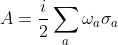
wobei die Pauli-Matrizen als Generatoren und die omegas als Rotationsparameter auftreten.
Für beliebige zeitabhängige Rotation d.h. zeitabhängige omegas integriert man die Bewegungsgleichung für U(t) mit der Anfangsbedingung U(0) = 1
=%5Ctext%7BT%7D%5C,%5Ctext%7Bexp%7D%5C,%5Cint_0%5Et&space;ds%5C,A(s))
Möchte man über kurze jedoch nicht-infinitesimale Zeitintervalle integrieren, so kann man die weiter oben genannten Methoden analog zu RK4 einführen; ich verzichte zunächst mal darauf. Das zeitgeordnete Produkt ist ein Element der SU(2) mit der Eigenschaft
=U(t_2,t_i)%5C,U(t_i,t_1))
Insbs. gilt
=%5Clim_%7BN%5Cto%5Cinfty%7D%5C;%5Cprod_%7Bn=1%7D%5EN%5C,U_n,%5Cqquad&space;U_n=e%5E%7BA_n%5C,%5CDelta&space;t_n%7D)
wobei A_n die zum Zeitpunkt t_n vorliegende Rotation gemäß omega, und Delta t_n das jeweilige Zeitintervall bezeichnet.
Die Lösung für den Vektor X(t) folgt dann wie oben, für ein iteratives Vorgehen je neuem Zeitschritt zu

Das Schöne an der Darstellung ist, dass man einfach je Zeitschritt mit der infinitesimalen Rotation multiplizieren kann, dass die Norm automatisch erhalten ist, und dass U bzw. A unmittelbar aus omega folgen. Eine Umrechnung zwischen verschiedenen Koordinatensystemen und Darstellungen ist nicht notwendig (falls man omega direkt verwenden darf, wovon ich immer ausgegangen bin; falls das nicht zutrifft, geht ein wesentlicher Vorteil verloren). Ein Nachteil besteht ggf. darin, dass die Einführung von Methoden analog zu RK4 notwendig und aufwändig wird, und dass die kompakte Form zerbröselt. Allerdings könnten man tatsächlich jede Matrix je Schritt n dergestalt auffassen, die Mathematik ließe das zu.
In der von mir genannten Form muss das letztlich die von euch verwendete Integration der Bewegungsgleichung mittels Quaternionen sein, denn die Entsprechung zwischen su(2) & SU(2) sowie Quaternionen ist eins-zu-eins; ich habe da sicher nichts neues entdeckt.
D.h. man erhält diese drei Komponenten der Winkelgeschwindigkeit. Damit würde mein Programm klarkommen.
Aber: bzgl. welches Koordinatensystems erhält man diese drei Komponenten? Bzgl. eines in guter Näherung infertialen System, oder bzgl. eines mitrotierende Systems? Für mich ergibt nur erstens Sinn.
TomS
Registriertes Mitglied
Ich habe jetzt nochmal eine zweite Parametrisierung der unitären Transformation eingebaut, nämlich
Das führt zu keinen wesentlich anderen Ergebnissen., dU/dt ist "gutartig".
Ein Hinweis: ich habe meine Matrizen immer so gewählt, dass U(t)1) = 1 ist. Damit sollte der Vektor eigentlich zum Ausgangspunkt zurückrotiert werden. Das ist aber nur ein Konsistenzcheck; maßgeblichen sind natürlich die Abweichungen für 0 < t < 1, die zeigen die numerischen Probleme.
Der nächste Schritt ist dann, das von C^2-Vektoren auf su(2) Matrizen = Quaternionen umzustellen, d.h.
Zur Gegenüberstellung noch folgendes: Bisher betrachtet ich
)
=\bar{Z}UZ&space;)
d.h. U rotiert Z, und das Skalaprodukt liefert für normiertes Z gerade den Rotationswinkel; der hängt natürlich von U und Z ab. Das ist ein natürliches Maß dafür, wie weit UZ von Z wegrotiert wurde. Man erhält das aus der FS-Metrik oder direkt. In meinem Plot nenne ich das "angle-distance".
Etwas ähnliches funktioniert auch, wenn man ein su(2)- bzw. quaternion-wertiges X betrachtet. Man verwendet dazu
=\frac{1}{2}\text{tr}XY=\frac{1}{2}\text{tr}\sum_{ab}x^a\sigma^a&space;y^b\sigma^b)
Für Produkt und Spur zweier Pauli-Matrizen gilt

und damit folgt letztlich

D.h. der zuerst genannte Ausdruck eines Skalarproduktes auf dem Vektorraum der Lie-Algebra su(2) entspricht direkt dem Skalarprodukt auf dem 3-dim. euklidischen Raum.
Der für normiertes X daraus folgende Rotationswinkel (zwischen X und Y) ist natürlich wiederum von X und U abhängig.
An der Stelle nochmal der Hinweis auf:
 en.wikipedia.org
wobei ich wieder nur die iterative Variante mit kleinen Zeitschritten betrachte.
Das führt zu keinen wesentlich anderen Ergebnissen., dU/dt ist "gutartig".
Ein Hinweis: ich habe meine Matrizen immer so gewählt, dass U(t)1) = 1 ist. Damit sollte der Vektor eigentlich zum Ausgangspunkt zurückrotiert werden. Das ist aber nur ein Konsistenzcheck; maßgeblichen sind natürlich die Abweichungen für 0 < t < 1, die zeigen die numerischen Probleme.
Der nächste Schritt ist dann, das von C^2-Vektoren auf su(2) Matrizen = Quaternionen umzustellen, d.h.
Die SU(2)-Matrizen U bleiben dieselben.
Zur Gegenüberstellung noch folgendes: Bisher betrachtet ich
d.h. U rotiert Z, und das Skalaprodukt liefert für normiertes Z gerade den Rotationswinkel; der hängt natürlich von U und Z ab. Das ist ein natürliches Maß dafür, wie weit UZ von Z wegrotiert wurde. Man erhält das aus der FS-Metrik oder direkt. In meinem Plot nenne ich das "angle-distance".
Etwas ähnliches funktioniert auch, wenn man ein su(2)- bzw. quaternion-wertiges X betrachtet. Man verwendet dazu
Für Produkt und Spur zweier Pauli-Matrizen gilt
und damit folgt letztlich
D.h. der zuerst genannte Ausdruck eines Skalarproduktes auf dem Vektorraum der Lie-Algebra su(2) entspricht direkt dem Skalarprodukt auf dem 3-dim. euklidischen Raum.
Der für normiertes X daraus folgende Rotationswinkel (zwischen X und Y) ist natürlich wiederum von X und U abhängig.
An der Stelle nochmal der Hinweis auf:
Pauli matrices - Wikipedia
Python:
# SU(2) orbits on the complex unit sphere

# imports ----------

import numpy as np
np.set_printoptions(threshold=np.inf)

import scipy as sci

import matplotlib.pyplot as plt
from matplotlib import use
use('MacOSX')
plt.rc('font', size=8)

import mplcyberpunk
plt.style.use("cyberpunk")


# S2, su(2) and SU(2) ----------

e_x = np.array([1.0, 0.0], dtype=complex)
e_y = np.array([0.0, 1.0], dtype=complex)

sigma_x = np.array([[0, 1], [1, 0]], dtype=complex)
sigma_y = np.array([[0, -1j], [1j, 0]], dtype=complex)
sigma_z = np.array([[1, 0], [0, -1]], dtype=complex)
sigma = np.array([sigma_x, sigma_y, sigma_z])

Id_2 = np.eye(2, dtype=complex)


# the model ----------

def hopf_rep(t,                                                                             # a specific motion, using Hopf-angle representation
             k=2, kappa=3.0,                                                                # winding number and steepness of angle theta
             a=0.5, b=1.7,                                                                  # amplitudes of angles phe_1 and phi_2
             omega_a=1.0, omega_b=3.3,                                                      # frequency of angles phi_1, phi_2
             delta_ab=0.6):                                                                 # phase shift
    s = 2 * t - 1
    theta = k * np.pi * (np.tanh(kappa * s) / np.tanh(kappa) + 1.0)                         # then three Hopf angles
    phi_a = a * np.pi * np.sin(omega_a * np.pi * t)**2
    phi_b = b * np.pi * np.sin(omega_b * np.pi * t)**2 - delta_ab
    z_a = np.exp(1j * phi_a) * np.cos(theta)                                                # the matrix elements
    z_b = np.exp(1j * phi_b) * np.sin(theta)
    U = np.array([[z_a, z_b], [-z_b.conj(), z_a.conj()]], dtype=complex)                    # the SU(2) matrix
    return U


def lie_rep(t,                                                                              # a specific motion, using Lie-algebra representation
            a=(0.7, 0.5, -0.1),
            o=(2.3, 1.1, -3.2),
            d=(0.3, 0.7, -1.2),
            s=1.3):
    a = np.asarray(a)
    o = np.asarray(o)
    d = np.asarray(d)

    trig_1 = np.cos(2 * np.pi * o * t - d) + s
    trig_2 = np.sin(np.pi * t)**2

    p = a * trig_1 * trig_2
    # A = p[0] * sigma_x + p[1] * sigma_y + p[2] * sigma_z
    A = np.tensordot(p, sigma, axes=1)
    U = sci.linalg.expm(1j * A * t)
    return U


# the SU(2) group and its su(2) algebra ----------

def rot_matrix(t, rot_func=lie_rep):                                                        # the SU(2) matrix
    return rot_func(t)


def gen_matrix(t, dt=1e-6):                                                                 # the su(2) matrix generating a small rotation
    U = rot_matrix(t)
    dU = (rot_matrix(t + dt) - rot_matrix(t - dt)) / (2 * dt)
    A = dU @ U.conj().T
    return A


def FS_dist(z_a, z_b):                                                                      # Fubini-Study-distance on the sphere
    overlap = (
        np.einsum('ij,ij->i', np.conj(z_a), z_b)
        if z_b.ndim == 2
        else np.einsum('ij,j->i', np.conj(z_a), z_b)
    )
    cos = np.abs(overlap)
    sqr_dist = 2 - 2 * cos
    angle = np.arccos(np.clip(np.abs(cos), 0.0, 1.0))
    return overlap, cos, angle, sqr_dist


# the solutions for dU/dt = AU: direct, step-wise linear, step-wise using matrix exponential ----------

def impl_exact(t_i, dt_i, z_prev, z_0):                                                     # z(t) = U(t) * z_0
    U_i = rot_matrix(t_i)
    z_i = U_i @ z_0
    z_i = z_i / np.linalg.norm(z_i)
    return z_i , U_i


def impl_iter_lin(t_i, dt_i, z_prev, z_0):                                                  # z(n+1) = (1 + A dt) * z(n)
    A_i = gen_matrix(t_i)
    z_i = (Id_2 + A_i * dt_i) @ z_prev
    z_i = z_i / np.linalg.norm(z_i)
    return z_i, A_i


def impl_Cayley_trf(t_i, dt_i, z_prev, z_0):                                                # z(n+1) = W^{-1} * V z(n);
    I = Id_2
    A_i = gen_matrix(t_i)
    V_i = I + A_i * dt_i / 2
    W_i = I - A_i * dt_i / 2
    z_i = np.linalg.solve(W_i, V_i @ z_prev)                                                # this solves W * z(n+1) = V * z(n)
    z_i = z_i / np.linalg.norm(z_i)
    return z_i, A_i


def impl_iter_exp(t_i, dt_i, z_prev, z_0):                                                  # z(n+1) = exp(A dt) * z(n)
    A_i = gen_matrix(t_i)
    z_i = sci.linalg.expm(A_i * dt_i) @ z_prev
    z_i = z_i / np.linalg.norm(z_i)
    return z_i, A_i


def calc_solution(t, z_0, N, impl_func):
    z = np.zeros((N, 2), dtype=complex)
    z[0] = z_0
    for i in range(1, N):
        t_i = t[i]
        dt_i = t[i] - t[i-1]
        z_i, M = impl_func(t_i, dt_i, z[i-1], z_0)
        z[i] = z_i
    return z, M                                                                             # this is either U_i or A_i


# the solutions ----------

N = 500
t = np.linspace(0.0, 1.0, N)

z_0 = e_x
z_lst = []
for impl_func in [impl_exact, impl_iter_lin, impl_Cayley_trf, impl_iter_exp]:
    z, _ = calc_solution(t, z_0, N, impl_func)
    z_lst.append(z)

overlap_lst = []
sqr_dist_list = []
for z in z_lst[1:]:
    overlap, cos, angle, sqr_dist = FS_dist(z, z_lst[0])
    overlap_lst.append(overlap)
    sqr_dist_list.append(sqr_dist)
    sqrt_I_angle_dist = np.sqrt(np.trapezoid(np.abs(angle), t))
    print(sqrt_I_angle_dist)


z = z_lst[0]
for k in range(2):
    plt.plot(z[:,k].real, z[:,k].imag, lw=0.5)
plt.gca().set_aspect('equal', adjustable='box')
plt.title('SU(2) orbit')
plt.show()


for txt, z in zip(['exact', 'lin iter', 'Cayley iter', 'exp iter'], z_lst):
    overlap, cos, angle, sqr_dist = FS_dist(z, z_0)
    plt.scatter(t, angle, s=0.25, label=txt)
plt.title('solutions, angle-distance from starting point, using Fubini-Study metric')
plt.legend()
plt.show()


for txt, overlap in zip(['lin iter', 'Cayley iter', 'exp iter'], overlap_lst):
    plt.plot(overlap.real - 1, overlap.imag, lw=0.5, label=txt)
plt.title('deviation of solutions, Fubini-Study-overlap with exact solution')
plt.legend()
plt.show()


for txt, sqr_dist in zip(['lin iter', 'Cayley iter', 'exp iter'], sqr_dist_list):
    plt.scatter(t, sqr_dist, s=0.25, label=txt)
plt.title('deviation of solutions, Fubini-Study-distance from exact solution')
plt.yscale('log')
plt.legend()
plt.show()
Zuletzt bearbeitet:

ralfkannenberg
Registriertes Mitglied
Ich nehme das mal so hin, ich würde aber gerne auch den Grund verstehen. Bei der Darstellung mittels Eulerwinkeln ist mir das Problem klar.
Hallo zusammen,Warum sollte das so sein? Das mag für die Darstellung mittels Eulerwinkeln so sein, aber welche Größe friert bei Quaternionen ein? Oder welche kann unendlich werden?
ich habe etwas den Überblick verloren. Sind diese beiden Probleme inzwischen gelöst ?
Freundliche Grüsse, Ralf
TomS
Registriertes Mitglied
Ja.Sind diese beiden Probleme inzwischen gelöst ?
Das Problem ist folgendes: du möchtest eine beliebige Rotation mittels dreier einzelner Rotationen um zwei oder drei vorab festgelege, paarweise orthogonale Achsen durchführen, z.B. Luftfahrt mit Abfolge Gieren-Nicken-Rollen zyx, oder klassisch Mechanik mit Eulerwinkeln zxz.
Durch die feste Achsenabfolge existieren Fälle, in denen zwei der Rotationsachsen parallel ausgerichtet werden, so dass in der Folge statt einer SO(3)- nur noch eine SO(2)-Rotation möglich ist. Das System hat einen Freiheitsgrad verloren.
Die zuletzt verlinkten Videos zeigen das Problem sehr anschaulich.
Mechanisch kann man das Problem durch mehrere einzelne Rotationen plus dynamische Änderung der Reihenfolge der Achsen oder einer vierten Hilfsachse in den Griff bekommen.
Mathematisch löst man das Problem mittels Rotationen von Quaternionen = su(2)-Matrizen oder komplexer 2-Spinoren. Das läuft einfach darauf hinaus, dass man die gewünschte Rotationen SO(3) ~ SU(2) durch eine feste Drehachse und den zugehörigen Winkel darstellt.
In 3 Dimensionen ist das eindeutig, da Start- und Zielvektor eindeutig eine Ebene und damit eine dazu senkrechte Rotationsachse definieren. In 4 Dimensionen haben wir den Spezialfall SO(4) ~ SU(2) * SU2). In n > 4 sind die n - 2 > 2 Rotationsachsen nicht eindeutig, jedoch weiterhin die 2-dim. Rotationsebene …
albertus
Registriertes Mitglied
Hallo zusammen, die Diskussion hat durch Toms Erläuterung zum Gimbal Lock und den Verweis auf die Videos eine tolle Tiefe bekommen. Für mich als Elektroniker wird hier der entscheidende Vorteil der Quaternionen (und damit der SU(2)-Mathematik) gegenüber den klassischen Euler-Winkeln kristallklar:
Es geht nicht nur um mathematische Eleganz, sondern um Betriebssicherheit. In der Luft- und Raumfahrt ist der 'Gimbal Lock' der Super-GAU – ein Zustand, in dem die Steuerung einen Freiheitsgrad verliert, weil sich zwei Achsen überlagern. Dass die SU(2)-Matrix (oder das Quaternion) diesen Zustand prinzipiell gar nicht kennt, macht sie zur 'Versicherungspolice' für jeden Satelliten.
Mein nächster Schritt bei der Einarbeitung ist nun die Praxis der Umrechnung. Wenn wir – wie TomS fragte – die Rohdaten der Sensoren (Winkelgeschwindigkeiten
 ,
,
 ) bekommen, müssen wir diese stabil integrieren. Die Videos von 3Blue1Brown zeigen wunderbar, warum wir dabei mit dem halben Winkel
 arbeiten.
Genau hier treffen sich Theorie und Hardware:
Es geht nicht nur um mathematische Eleganz, sondern um Betriebssicherheit. In der Luft- und Raumfahrt ist der 'Gimbal Lock' der Super-GAU – ein Zustand, in dem die Steuerung einen Freiheitsgrad verliert, weil sich zwei Achsen überlagern. Dass die SU(2)-Matrix (oder das Quaternion) diesen Zustand prinzipiell gar nicht kennt, macht sie zur 'Versicherungspolice' für jeden Satelliten.
Mein nächster Schritt bei der Einarbeitung ist nun die Praxis der Umrechnung. Wenn wir – wie TomS fragte – die Rohdaten der Sensoren (Winkelgeschwindigkeiten
Genau hier treffen sich Theorie und Hardware:
- Die Pauli-Matrizen bilden das mathematische Gerüst (die Basis).
- Die Quaternionen sind das kompakte Werkzeug für die Rotation.
- Die Cayley-Transformation (die TomS in seinem Programm nutzt) sorgt dafür, dass die numerischen Rundungsfehler uns nicht vom Kurs abbringen.
TomS
Registriertes Mitglied
Bisher habe ich folgendes:
Hier ein Ergebnis der Runs:
Dabei sieht man die Run-Nummer mit dem größten Fehler: 71389 (von 100000). Die Matrix zählt die Aufrufe der Umrechnungen
- reelle 3er Vektoren
- komplexe 2er Spionieren (Hopf-Abbildung)
- komplexe su(2)-Matrizen (mittels Pauli-Matrizen)
- jeweils bijektive Abbildung
- jeweils Skalarprodukt und Norm
- Rotationen für diese drei Abbildungen, immer ausgehend von einem 3er-Vektor für Omega, dann Berechnung und Anwendung von R als SO(3) und U als SU(2) Matrix
- 100000 Runs
- je Run 16 Wechsel der Repräsentation (3er V., 2er S., su(2)) sowie 8 Rotationen; dabei dt = 1e-3 sek.
- ich teste dabei immer zwei unterschiedliche Zufallsvektoren mit unterschiedlichen Wechseln der Darstellungen jedoch identischen Omegas
- dabei lande ich meistens bei Fehlern im Bereich 1-e5 oder besser, manchmal schlägt jedoch die Numerik zu, ich weiß nicht nicht wo
- 100000 Runs
- je Run wie oben, jedoch kein Reset, d.h. effektiv 100000 * 16 * 8 Berechnungen
- Fehler teilw. wie oben, manchmal bei 1e-12, jedoch gibt es manchmal deutliche Ausreißer
- Fehler je Repräsentation untersuchen, d.h. keine Umrechnung zwischen denselben
- Effekte des Samplings von Omega und der Anfangsbedingungen verstehen
- gezielt kritische Punkte untersuchen (die Abbildung auf die Spinor-Darstellung hat eine Singularität bei z=-1)
Python:
# library implementing functions for represenrting (rotations of) unit 3-vectors, also using 2-spinors and su(2) algebra

# ATTENTION:
# normalization of input data is assumed to be provided by caller, not enforced by callee
# normalization of output data is not enforced by callee, needs to be checked and enforced by caller

# imports ----------

import numpy as np
np.set_printoptions(threshold=np.inf)

from scipy.linalg import expm

# Pauli matrices ----------

sigma_x = np.array([[0, 1], [1, 0]], dtype=complex)
sigma_y = np.array([[0, -1j], [1j, 0]], dtype=complex)
sigma_z = np.array([[1, 0], [0, -1]], dtype=complex)

sigmas = np.array([sigma_x, sigma_y, sigma_z])

Id_2 = np.eye(2, dtype=complex)


# inner products  and norms ----------

# ⟨x, y⟩; works for x, y in arbitrary dimension x, y ∈ ⊂ ℝⁿ
def inner_vec(x, y):
    return np.dot(x, y)

def norm_vec(x):
    return np.sqrt(inner_vec(x, x))


# ⟨Z, W⟩; works for Z, W in arbitrary dimension Z, W ∈ ℂⁿ
def inner_spin_complex(Z, W):
    return np.vdot(Z, W)

# ⟨Z, W⟩; projected from to ℂ²) ⊂ ℂ² ~ S³ / U(1) ~ S² to mathc Hopf / Fubini-Study
def inner_spin(Z, W):
    return np.real( 2 * np.abs(np.vdot(Z, W))**2 - np.vdot(Z, Z) * np.vdot(W, W) )

def norm_spin(Z):
    return np.sqrt(inner_spin(Z, Z))


# ⟨X, Y⟩; works in arbitrary dimensions X, Y ∈ su(n), provided a) fundamental representation and b) Pauli-like normalization
def inner_su2(X, Y):
    return 0.5 * np.real(np.trace(X @ Y))

def norm_su2(X):
    return np.sqrt(np.real(inner_su2(X, X)))


# ----------
# maps between
# normed 3-vector x ∈ S² ⊂ ℝ³
# normed 2-spinor Z ∈ S(ℂ²) ⊂ ℂ² ~ S³ ⊂ ℝ⁴, and
# normed X ∈ S(su(2)) ⊂ su(2)

# x ⟶ Z; inverse Hopf map with choice of section x³ ≠ -1)
def vec_to_spin(x):
    if 1 + x[2] < 1e-6:
        print(f'warning z-component {x[2]} causes spinor-singularity')
        return np.array([0.0, 1.0], dtype=complex)

    z1 = np.sqrt((1 + x[2]) / 2)
    z2 = (x[0] + 1j * x[1]) / np.sqrt(2 * (1 + x[2]))
    Z = np.array([z1, z2], dtype=complex)
    return Z


# Z ⟶ x; Hopf-map
def spin_to_vec(Z):
    x = np.array([np.vdot(Z, sigmas[i] @ Z) for i in range(3)])
    return np.real(x)


# x ⟶ X
def vec_to_su2(x):
    x1, x2, x3 = x
    X = np.array([
        [x3,            x1 - 1j * x2],
        [x1 + 1j * x2, -x3]
    ], dtype=complex)
    return X


# X ⟶ x
def su2_to_vec(X):
    x = np.array([0.5 * np.real(np.trace(X @ sigmas[i])) for i in range(3)])
    return x


# Z ⟶ X
def spin_to_su2(Z):
    Z = np.asarray(Z, dtype=complex).reshape(2, 1)
    X = 2.0 * Z @ Z.conj().T - Id_2
    return X

# X ⟶ Z
def su2_to_spin(X):
    P = 0.5 * (X + Id_2)
    vals, vecs = np.linalg.eigh(P)
    Z = vecs[:, np.argmax(np.real(vals))]
    return Z


# rotation matrices R(ω, dt) ∈ SO(3) and U(ω, dt) ∈ su(2) ----------

# R = exp(dt * Ω) ∈ SO(3), using # skew-symmetric matrix Ω ∈ so(3) derived from ω
def omega_to_vecrot(omega, dt):
    w1, w2, w3 = omega
    Omega = np.array([
        [0, -w3, w2],
        [w3, 0, -w1],
        [-w2, w1, 0]
    ], dtype=float)
    return expm(dt * Omega)


# U = exp(-i/2 dt ω·σ) ∈ SU(2)
def omega_to_SU2rot(omega, dt):
    w1, w2, w3 = omega
    A = np.array([
        [w3,            w1 - 1j * w2],
        [w1 + 1j * w2, -w3]
    ], dtype=complex)
    return expm(-0.5j * dt * A)


# apply rotations ----------

# x ⟶ R x
def rotate_vec(omega, x, dt):
    R = omega_to_vecrot(omega, dt)
    y = R @ x
    return y


# Z ⟶ U Z
def rotate_spin(omega, Z, dt):
    U = omega_to_SU2rot(omega, dt)
    W = U @ Z
    return W


# X ⟶ U X U⁺
def rotate_su2(omega, X, dt):
    U = omega_to_SU2rot(omega, dt)
    V = U @ X @ U.conj().T
    return V
Python:
# tester

import numpy as np
import random as rnd

import mcu_lib as mcu


# classifies representations according to numpy arrays, using 'real 3-vec': 0; 'complex 2-spin': 1, 'complex su(2): 2
def rep_code(p: np.ndarray):
    shape = p.shape
    kind = p.dtype.kind  # 'f' float, 'c' complex, 'i' int, etc.

    if shape == (3,) and kind == 'f':
        return 0
    elif shape == (2,) and kind == 'c':
        return 1
    elif shape == (2, 2) and kind == 'c':
        return 2
    else:
        raise ValueError(f'Unsupported representation: {shape, kind}')


# dispatches all inner product calls
def inner(p, q):
    rpc_p = rep_code(p)
    rpc_q = rep_code(q)
    if rpc_p != rpc_q:
        raise ValueError(f"Incompatible representations: {rpc_p}, {rpc_q}")

    if rpc_p == 0:
        return mcu.inner_vec(p, q)
    if rpc_p == 1:
        return mcu.inner_spin(p, q)
    if rpc_p == 2:
        return mcu.inner_su2(p, q)


# dispatches all rotations calls
def rotate(omega, p, dt=1e-03):
    rpc_p = rep_code(p)

    if rpc_p == 0:
        return mcu.rotate_vec(omega, p, dt)
    if rpc_p == 1:
        return mcu.rotate_spin(omega, p, dt)
    if rpc_p == 2:
        return mcu.rotate_su2(omega, p, dt)


def id(p):
    return p

rep_map = [
    [id,                mcu.vec_to_spin,    mcu.vec_to_su2],
    [mcu.spin_to_vec,   id,                 mcu.spin_to_su2],
    [mcu.su2_to_vec,    mcu.su2_to_spin,    id]
]

call_stat = np.zeros_like(rep_map, dtype=int)

# maps input p to new representation rpc_new
def map_rep(p, rpc_new):
    rpc = rep_code(p)
    call_stat[rpc, rpc_new] += 1
    return rep_map[rpc][rpc_new](p)


# generate all rep-schedules of length N
def get_rep_scheds(N):
    if N < 1:
        return []

    rep_codes = [0, 1, 2]

    def backtrack(current):
        if len(current) == N:
            return [current.copy()]
        results = []
        last = current[-1]
        for rpc in rep_codes:
            if rpc != last:
                current.append(rpc)
                results.extend(backtrack(current))
                current.pop()
        return results

    return backtrack([0])


# generate all rotation schedules of length N
def get_om_scheds(om, N):
    L = len(om)

    # weak compositions of L into N parts
    def compositions(L, N):
        if N == 0:
            if L == 0:
                return [[]]
            return []
        if N == 1:
            return [[L]]

        result = []
        for first in range(L + 1):
            for rest in compositions(L - first, N - 1):
                result.append([first] + rest)
        return result

    # convert length-partition -> actual slices
    def slices_from_lengths(lengths):
        out = []
        i = 0
        for l in lengths:
            out.append(om[i:i + l])
            i += l
        return out

    return [slices_from_lengths(lengths) for lengths in compositions(L, N)]


# randomly scaled, randomly distributed unit 3-vectors
def get_scaled_unit_vectors(N, scale=None):
    vecs = np.random.standard_normal(size=(N, 3))
    vecs /= np.linalg.norm(vecs, axis=1, keepdims=True)
    if scale:
        scales = np.random.uniform(0, scale, size=(N, 1))
        vecs = scales * vecs
    return list(vecs)


# exectutes one test run for one pait auf schedules
def run(p, rep_scheds, om_scheds):
    rpcs = rnd.sample(rep_scheds, 1)[0]
    oms = rnd.sample(om_scheds, 1)[0]
    for rpc_new, om in zip(rpcs, oms):
        p = map_rep(p, rpc_new)
        for o in om:
            p = rotate(o, p)
            p /= np.sqrt(inner(p, p))
    return p


RUNS = 100000

SCHED_LEN = 16
NUM_ROT = 8

omegas = get_scaled_unit_vectors(NUM_ROT, scale=3.0)

rep_scheds = get_rep_scheds(SCHED_LEN)
om_scheds = get_om_scheds(omegas, SCHED_LEN)

print(len(rep_scheds), len(om_scheds))

x, y = get_scaled_unit_vectors(2, None)
ipr_xx, ipr_yy, ipr_xy = inner(x, x), inner(y, y), inner(x, y)

p = x.copy()
q = y.copy()

max_dev = -np.inf
for r in range(RUNS):
    p = run(p, rep_scheds, om_scheds)
    q = run(q, rep_scheds, om_scheds)

    p_r = map_rep(p, 0)
    q_r = map_rep(q, 0)

    dev = np.max(np.abs([inner(p_r, p_r) - ipr_xx, inner(q_r, q_r) - ipr_yy, inner(p_r, q_r) - ipr_xy]))
    if dev > max_dev:
        max_dev = dev
        print(r, dev)

print(call_stat)
Hier ein Ergebnis der Runs:
Code:
71389 1.8868636098012814e-08
[[133784 544672 544178]
 [611944      0 477444]
 [610014 477964      0]]
Dabei sieht man die Run-Nummer mit dem größten Fehler: 71389 (von 100000). Die Matrix zählt die Aufrufe der Umrechnungen
Zuletzt bearbeitet:
albertus
Registriertes Mitglied
Warum Tom diesen Aufwand treibt
Vielleicht fragt ihr euch: „Warum simuliert Tom 100.000 Flugmanöver? Haben die Raumfahrtingenieure das nicht schon vor Jahrzehnten erledigt?“Die Antwort lautet: Ja, absolut. Aber in der Raumfahrt liest man von diesen Tests kaum etwas, weil sie in den „Pre-Flight-Checks“ stattfinden. Bevor eine Software eine Rakete steuert, wird sie „gequält“. Tom hat diesen unsichtbaren Prozess für seine Bibliothek mcu_lib.py nachgeholt. Er zeigt uns damit, dass unsere Werkzeuge nicht nur auf dem Papier existieren, sondern unter extremer digitaler Last bestehen.
Was uns der Härtetest beweist
In der Theorie ist die SU(2)-Mathematik (die Basis für unsere Quaternionen-Steuerung) perfekt. Aber ein Computer kennt keine unendliche Präzision. Er hat nur Nachkommastellen. Bei jeder Drehung und jedem Wechsel der Darstellung „schneidet“ der Prozessor ein winziges Stückchen Genauigkeit ab.Toms Test zeigt, dass die Berechnungen extrem stabil bleiben, solange wir die „numerischen Leitplanken“ einhalten. In meinen eigenen Testläufen mit 1.000 Iterationen blieben die Fehler konstant im Bereich von
Die konkreten Leitplanken in unserem Code:
- Die ständige Re-Normierung (Der Kampf gegen den „Zollstock-Effekt“):
Durch winzige Rundungsfehler werden Quaternionen im Speicher ganz langsam „länger“ oder „kürzer“ als 1,0. In der Realität würde das bedeuten, dass das Raumschiff rechnerisch plötzlich „anschwillt“.- Die Leitplanke: Der Code zwingt das Ergebnis nach jedem Schritt zurück auf die Länge 1,0 (p /= np.sqrt(inner(p, p))). Das ist das „Geraderücken“ der physikalischen Realität im Rechner.
- Das Meiden der Singularität (Die „Südpol-Klippe“):
Wie Tom im Log zeigt, gibt es einen Punkt (den „Südpol“ bei z = -1), an dem die mathematische Formel für die Spinoren theoretisch durch Null teilen müsste.- Die Leitplanke: Ein robuster Algorithmus muss erkennen, wenn man sich diesem Punkt nähert. Toms 100.000 Runs provozieren diese kritischen Momente absichtlich, um sicherzustellen, dass das System nicht unkontrolliert abstürzt, sondern berechenbar bleibt.
- Das numerische Grundrauschen:
Diese Tests legen fest, wie oft wir einen Sternensensor zur Korrektur brauchen. Wenn wir wissen, wie schnell die Mathematik „driftet“, wissen wir, wie oft wir die reale Position abgleichen müssen.
Fazit für unser Projekt
Toms „Bahnhof aus Zahlen“ ist das Sicherheitssiegel für unser Forum. Er hat bewiesen: Unsere SU(2)-Implementierung hält auch nach 1.600.000 Rechenoperationen die Spur. Wir präsentieren hier keine „Heimwerker-Lösung“, sondern eine mathematisch geprüfte Basis, die theoretisch reif für den Orbit wäre. Diese Stabilität ist die Voraussetzung dafür ist, dass man sich auf die Quaternionen-Regelung auch bei Langzeitmissionen verlassen kann.
TomS
Registriertes Mitglied
Na ja, was ich gemacht habe, war nur der Einstieg, ich kratze sozusagen an der Oberfläche. Mein Ziel war, einige Hürden besser zu verstehen. Die eigtl. Arbeit steckt in dem unscheinbaren expm(…), das ich einfach so nutze, und der Arbeit der Mathematiker über viele Jahrzehnte.
Ich habe noch vor …
Die Singularität ist nur problematisch, wenn man von x nach Z umrechnet. Für die Lösung in Z und die Umrechnung nach x ist alles regulär.
Noch eine Anmerkung: man wird wohl nie ein fettes Python-Script auf Interpreterbasis in einen Satelliten stecken, ich vermute, dass compilierter Code das Mittel der Wahl ist.
Ich habe noch vor …
- … eine bekannte Lösung für das Trudeln anzusetzen und zu prüfen, wie die Software sich da verhält
- … die Anfangsbedingungen und den Input für die komplexen Spinoren auf die Nordhalbkugel einzuschränken; die Lösung ist auch dann um einige Größenordnungen (!) schlechter, wenn man überhaupt nicht in den kritischen Bereich gelang; und das verstehe ich nicht
- … die gesamten dynamischen Gleichungen zu lösen …
Die Singularität ist nur problematisch, wenn man von x nach Z umrechnet. Für die Lösung in Z und die Umrechnung nach x ist alles regulär.
Noch eine Anmerkung: man wird wohl nie ein fettes Python-Script auf Interpreterbasis in einen Satelliten stecken, ich vermute, dass compilierter Code das Mittel der Wahl ist.
Der Code ist nur theoretisch reif für die Praxis, aber man bekommt extrem schnell ein gutes Gefühl, ob ein Ansatz funktionieren kann, oder nicht. Dafür ist eine Sprache wie Python optimal.Wir präsentieren hier keine „Heimwerker-Lösung“, sondern eine mathematisch geprüfte Basis, die theoretisch reif für den Orbit wäre. Diese Stabilität ist die Voraussetzung dafür ist, dass man sich auf die Quaternionen-Regelung auch bei Langzeitmissionen verlassen kann.
TomS
Registriertes Mitglied
Noch ein paar Kleinigkeiten:
Für numerische Integration mit Zeitschritten dt = 1e-3 sind alle Ansätze so stabil, dass keine abschließende Normierung notwendig ist; das liegt daran, dass sowohl die SO(3) als auch die SU(2) Matrix normerhaltend sind; es verhielte sich anders, wenn man die lineare Form statt des Matrixexponentials zur Integration nutzen würde; die lineare Form ist noch nicht in der Library enthalten.
Die Performance ist für alle drei Methoden ziemlich identisch: für eine Integration entlang von 1000000 Zeitschritten, d.h. 1000 Sekunden läuft der Integrator ca. 5.2, 6.0 bzw. 6.7 Sekunden für 3-dim. Vektoren, 2-dim. Spins und su(2)-Matrizen = Quaternionen. (d.h. grob gesprochen, verglichen mit Echtzeit benötigt nicht mal 1 % der CPU-Zeit).
Genauigkeit und Stabilität sind in allen Fällen ok; am schlechtesten schneidet die SU(2) auf 2-dim. komplexen Spins ab. Die Ursache liegt wohl darin, dass für |Z| = 1 die verbleibende Mannigfaltigkeit 3-dim. ist, während für 3-dim. Vektoren mit |x| = 1 sowie analog für su(2)-Matrizen mit |ω·σ| = 1 die Mannigfaltigkeiten nur 2-dim. sind
Man landet also immer wieder bei der su(2) bzw. den Quaternionen.
Für numerische Integration mit Zeitschritten dt = 1e-3 sind alle Ansätze so stabil, dass keine abschließende Normierung notwendig ist; das liegt daran, dass sowohl die SO(3) als auch die SU(2) Matrix normerhaltend sind; es verhielte sich anders, wenn man die lineare Form statt des Matrixexponentials zur Integration nutzen würde; die lineare Form ist noch nicht in der Library enthalten.
Die Performance ist für alle drei Methoden ziemlich identisch: für eine Integration entlang von 1000000 Zeitschritten, d.h. 1000 Sekunden läuft der Integrator ca. 5.2, 6.0 bzw. 6.7 Sekunden für 3-dim. Vektoren, 2-dim. Spins und su(2)-Matrizen = Quaternionen. (d.h. grob gesprochen, verglichen mit Echtzeit benötigt nicht mal 1 % der CPU-Zeit).
Genauigkeit und Stabilität sind in allen Fällen ok; am schlechtesten schneidet die SU(2) auf 2-dim. komplexen Spins ab. Die Ursache liegt wohl darin, dass für |Z| = 1 die verbleibende Mannigfaltigkeit 3-dim. ist, während für 3-dim. Vektoren mit |x| = 1 sowie analog für su(2)-Matrizen mit |ω·σ| = 1 die Mannigfaltigkeiten nur 2-dim. sind
Man landet also immer wieder bei der su(2) bzw. den Quaternionen.
albertus
Registriertes Mitglied
Hallo Tom, da liegst du völlig richtig mit deiner Vermutung: C++ ist tatsächlich der Standard und das Mittel der Wahl in der Satellitentechnik.
Der Grund ist simpel: In einem Satelliten zählen Performance und absolute Kontrolle über den Speicher. Ein Python-Interpreter wäre dort viel zu hungrig und zu langsam für die harten Echtzeitanforderungen. Aber wie du schon sagst: In C++ dauert alles um ein Vielfaches länger. Man muss dort oft die mathematischen Werkzeuge, die uns Python mit einem Befehl wie expm() oder np.linalg.eig() schenkt, mühsam selbst implementieren oder spezialisierte Bibliotheken einbinden.
Genau deshalb ist unser aktueller Weg so wertvoll. Wir nutzen Python als ‚High-Level-Prüfstand‘. Wir können hier in Rekordzeit prüfen, ob die Logik der SU(2)-Transformationen hält, bevor man überhaupt daran denkt, den extrem aufwendigen Weg in Richtung C++ für die Flugsoftware zu gehen. Python ist sozusagen unser mathematisches Windkanal-Modell.
Der Grund ist simpel: In einem Satelliten zählen Performance und absolute Kontrolle über den Speicher. Ein Python-Interpreter wäre dort viel zu hungrig und zu langsam für die harten Echtzeitanforderungen. Aber wie du schon sagst: In C++ dauert alles um ein Vielfaches länger. Man muss dort oft die mathematischen Werkzeuge, die uns Python mit einem Befehl wie expm() oder np.linalg.eig() schenkt, mühsam selbst implementieren oder spezialisierte Bibliotheken einbinden.
Genau deshalb ist unser aktueller Weg so wertvoll. Wir nutzen Python als ‚High-Level-Prüfstand‘. Wir können hier in Rekordzeit prüfen, ob die Logik der SU(2)-Transformationen hält, bevor man überhaupt daran denkt, den extrem aufwendigen Weg in Richtung C++ für die Flugsoftware zu gehen. Python ist sozusagen unser mathematisches Windkanal-Modell.